
Introduction to Linear Regression
Linear regression is a foundational statistical technique used for modeling the relationship between a dependent variable and one or more independent variables. It is widely applied in various domains such as economics, finance, healthcare, marketing, and more. In this comprehensive guide, we will delve deep into understanding linear regression, its variants, hands-on examples using Python, real-world use cases, and common interview questions related to linear regression.
Understanding Linear Regression
What is Linear Regression?
Linear regression is a statistical method that aims to model the relationship between a dependent variable (Y) and one or more independent variables (X) by fitting a linear equation to observed data. The goal is to find the best-fitting straight line that minimizes the sum of squared differences between the actual and predicted values.
Simple Linear Regression
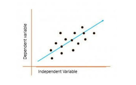
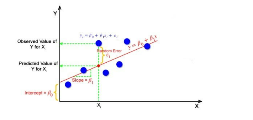
In simple linear regression, there is a single independent variable X and a single dependent variable Y. The relationship between X and Y is assumed to be linear, following the equation:
𝑌=𝛽0+𝛽1𝑋+𝜀Y=β0+β1X+ε
Where:
- Y is the dependent variable.
- X is the independent variable.
- β0 is the intercept (value of Y when X is 0).
- β1 is the slope of the line (change in Y for a unit change in X).
- ε represents the error term.
Hands-on Example: Simple Linear Regression in Python
Let’s demonstrate simple linear regression using Python to predict student scores based on study hours.
 #Importing libraries
import numpy as np
import pandas as pd
import matplotlib.pyplot as plt
from sklearn.linear_model import LinearRegression
from sklearn.model_selection import train_test_split

# Sample data (Study hours as X and Exam scores as Y)
data = {'StudyHours': [2, 4, 6, 8, 10],
        'ExamScores': [60, 65, 70, 75, 80]}
df = pd.DataFrame(data)

# Splitting data into training and testing sets
X_train, X_test, y_train, y_test = train_test_split(df[['StudyHours']], df['ExamScores'], test_size=0.2, random_state=42)

# Creating and fitting the model
model = LinearRegression()
model.fit(X_train, y_train)

# Making predictions
y_pred = model.predict(X_test)

# Evaluating the model
print("Coefficients:", model.coef_)
print("Intercept:", model.intercept_)
print("R-squared:", model.score(X_test, y_test))
Multiple Linear Regression
In multiple linear regression, there are multiple independent variables X1, X2, …, Xn predicting a single dependent variable Y. The equation takes the form:
𝑌=𝛽0+𝛽1𝑋1+𝛽2𝑋2+…+𝛽𝑛𝑋𝑛+𝜀Y=β0+β1X1+β2X2+…+βnXn+ε
This method is applicable when there are multiple factors influencing the outcome.
Use Case: House Price Prediction
Consider predicting house prices based on features like square footage, number of bedrooms, and location. Multiple linear regression can be employed for this predictive task.
Logistic Regression
While linear regression is used for continuous outcomes, logistic regression is suitable for binary classification problems. It predicts the probability that an instance belongs to a particular class.
Use Case: Email Spam Classification
In email spam classification, logistic regression can predict whether an email is spam (1) or not spam (0) based on features like keywords, sender’s address, and email content.
Gradient Descent for Optimization
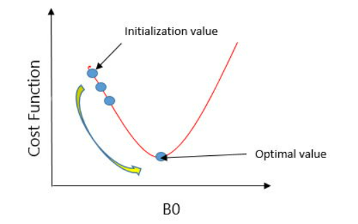
Gradient descent is an optimization algorithm used to minimize the cost function in linear regression. It iteratively adjusts model parameters to reach the optimal solution.
Understanding Gradient Descent
Gradient descent involves calculating gradients (partial derivatives) of the cost function with respect to model parameters and updating parameters in the opposite direction of the gradient.
Hands-on Example: Gradient Descent in Linear Regression
Let’s implement gradient descent for a simple linear regression problem in Python.
# Implement gradient descent for linear regression
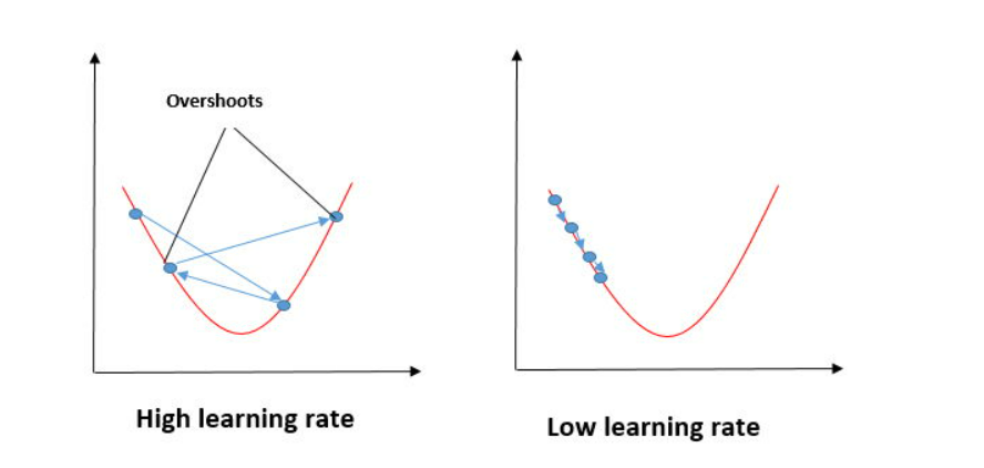
def gradient_descent(X, y, learning_rate=0.01, epochs=100):
m = len(y)
theta = np.zeros((2,1)) # Initialize parameters (theta0 and theta1)
X_b = np.c_[np.ones((m, 1)), X] # Add bias term to X
for epoch in range(epochs):
gradients = 2/m * X_b.T.dot(X_b.dot(theta) - y)
theta = theta - learning_rate * gradients
return theta
# Sample data
X = np.array([[1], [2], [3]])
y = np.array([[2], [4], [6]])
# Apply gradient descent
theta = gradient_descent(X, y)
print("Optimal parameters (theta0, theta1):", theta.ravel())
Evaluating Linear Regression Models
Metrics for Evaluation
- Mean Squared Error (MSE): Measures average squared difference between actual and predicted values.
- R-squared (Coefficient of Determination): Indicates the proportion of variance explained by the model.
Overfitting and Underfitting
- Overfitting: Occurs when the model learns noise in the training data, leading to poor generalization.
- Underfitting: Model is too simple to capture the underlying patterns in the data.
Real-world Use Cases of Linear Regression
- Financial Forecasting: Predicting stock prices based on historical data and market trends.
- Marketing ROI: Estimating sales based on advertising expenditure across different channels.
- Healthcare Analytics: Predicting patient outcomes based on medical history and treatment variables.
- Customer Lifetime Value: Estimating the lifetime value of a customer based on past behavior and demographics.
Interview Questions on Linear Regression
1. What are the assumptions of linear regression?
- Linearity
- Independence of residuals
- Homoscedasticity (Equal variance of residuals)
- Normality of residuals
2. How do you handle multicollinearity in linear regression?
- Using techniques like Variance Inflation Factor (VIF) to detect and remove highly correlated variables.
3. What is the difference between R-squared and adjusted R-squared?
- R-squared measures the proportion of variance explained by the model, while adjusted R-squared penalizes for adding unnecessary predictors.
4. Explain the bias-variance tradeoff in the context of linear regression.
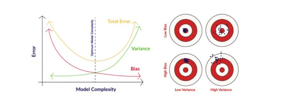
- Bias refers to errors from overly simplistic models, while variance refers to sensitivity to fluctuations in the training data. Balancing these is crucial for model generalization.
5. How do you evaluate the performance of a linear regression model?
- Using metrics such as R-squared, Root Mean Squared Error (RMSE), Mean Absolute Error (MAE), and visualizations like residual plots.
Conclusion
Linear regression is a powerful statistical technique with wide-ranging applications in predictive modeling and data analysis. By understanding its principles, implementing algorithms like gradient descent, exploring real-world use cases, and preparing for related interview questions, you can enhance your data science skills and excel in machine learning tasks involving linear regression. Keep practicing and experimenting with different datasets to master linear regression and its variants!
Visit : Movie Recommendations with Python
Visit : Stock Sentiment Analysis with machine learning and python