Logistic Regression serves as a fundamental technique in machine learning for binary and multi-class classification tasks. In this comprehensive guide, we’ll delve deep into Logistic Regression, starting from its basic concepts, types, assumptions, and gradually moving towards advanced topics like model interpretation, implementation using Python code examples, decision boundaries, cost function, gradient descent, model evaluation techniques, and a hands-on example using the Iris dataset. By the end, you’ll have a thorough understanding of Logistic Regression, suitable for beginners and those looking to reinforce their knowledge.
Understanding Logistic Regression
What is Logistic Regression?
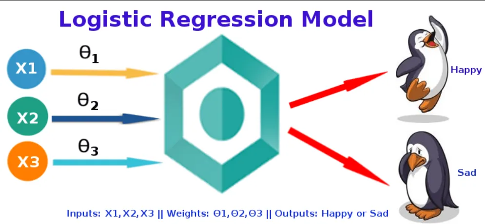
Logistic Regression is a supervised learning algorithm used for binary and multi-class classification tasks. Unlike Linear Regression, which predicts continuous values, Logistic Regression predicts the probability of an event occurring, assigning the input data to one of two or more possible categories based on a set of independent variables.
The Logistic Model
The logistic model transforms the linear regression output into probabilities using the logistic function (sigmoid function). The sigmoid function ensures that the output of the regression is mapped to probabilities between 0 and 1, making it suitable for classification tasks.
Types of Logistic Regression
- Binary Logistic Regression:
- Example: Predicting whether an email is spam (1) or not spam (0) based on features like keywords, sender, etc.
- Multinomial Logistic Regression:
- Example: Predicting the type of fruit (apple, banana, orange) based on features like color, size, and weight.
- Ordinal Logistic Regression:
- Example: Predicting customer satisfaction levels (low, medium, high) based on service ratings.
Assumptions of Logistic Regression
Logistic Regression relies on several assumptions:
- Minimal multicollinearity: Independent variables should not be highly correlated.
- Linear relationship: Log odds of the dependent variable should be linearly related to independent variables.
- Large sample size: Adequate data for reliable predictions.
- Independence of observations: Observations are assumed to be independent of each other.
- No influential outliers: Extreme values in predictors can skew results.
Why not Linear Regression for Classification?
Linear Regression isn’t suitable for classification due to its unbounded output range and inability to provide clear decision boundaries. Logistic Regression, with its sigmoid function, outputs probabilities between 0 and 1, making it ideal for classification tasks.
Advanced Concepts in Logistic Regression
Interpretation of Coefficients
In Logistic Regression, coefficients represent the log odds ratio change per unit change in the predictor. A positive coefficient indicates an increase in the odds of the event, while a negative coefficient indicates a decrease.
Odds Ratio and Logit
Odds ratio compares the odds of an event occurring with and without a particular variable. Logit is the natural logarithm of the odds ratio, often used for model interpretation.
Decision Boundary
The decision boundary separates classes in classification tasks. Logistic Regression finds an optimal boundary based on input features, aiding in accurate predictions.
Cost Function of Logistic Regression
The cost function measures the error between predicted probabilities and actual outcomes. It penalizes misclassifications and guides parameter updates during training. The commonly used cost function is the logistic loss (cross-entropy) function.
Gradient Descent in Logistic Regression
Gradient descent optimizes the cost function by iteratively updating model weights. It adjusts weights to minimize the cost and improve model accuracy. Proper learning rate selection and convergence monitoring are crucial for effective gradient descent.
Hands-on Example with the Iris Dataset
Let’s apply Logistic Regression to a real-world dataset to solidify our understanding. We’ll use the Iris dataset, a classic dataset in machine learning, containing features of iris flowers along with their species labels.
import numpy as np
import pandas as pd
from sklearn.datasets import load_iris
from sklearn.model_selection import train_test_split
from sklearn.preprocessing import StandardScaler
from sklearn.linear_model import LogisticRegression
from sklearn.metrics import accuracy_score, classification_report

# Load Iris dataset
iris_data = load_iris()
X = iris_data.data
y = iris_data.target

# Split data into training and testing sets
X_train, X_test, y_train, y_test = train_test_split(X, y, test_size=0.2, random_state=42)

# Standardize features
scaler = StandardScaler()
X_train_scaled = scaler.fit_transform(X_train)
X_test_scaled = scaler.transform(X_test)

# Initialize Logistic Regression model
log_reg_model = LogisticRegression(max_iter=1000, random_state=42)

# Train the model
log_reg_model.fit(X_train_scaled, y_train)

# Predictions on the test set
y_pred = log_reg_model.predict(X_test_scaled)

# Evaluate model performance
accuracy = accuracy_score(y_test, y_pred)
print(f"Accuracy: {accuracy:.4f}")

# Classification report
print("Classification Report:")
print(classification_report(y_test, y_pred, target_names=iris_data.target_names))
In this example, we:
- Load and preprocess the Iris dataset.
- Standardize features using
StandardScaler. - Train a Logistic Regression model on the training data.
- Evaluate the model’s accuracy and generate a classification report.
Model Evaluation in Logistic Regression
Model evaluation is crucial to assess its performance:
- Accuracy Score: Measures overall model accuracy on test data.
- Classification Report: Provides precision, recall, F1-score, and support for each class.
Overfitting
Definition: Overfitting occurs when a model learns the training data too well, capturing noise and random fluctuations rather than the underlying patterns. As a result, the model performs well on the training data but fails to generalize to new, unseen data.
Causes of Overfitting:
- Complex Models: Models with high complexity (too many parameters or features) can capture noise instead of patterns.
- Insufficient Data: When training data is limited, the model may memorize the training examples rather than learning generalizable patterns.
- Lack of Regularization: Without regularization techniques, models may become overly complex and prone to overfitting.
Signs of Overfitting:
- High Training Accuracy, Low Test Accuracy: The model performs exceptionally well on training data but poorly on test/validation data.
- High Variance: The model’s predictions vary significantly with small changes in the training data.
Prevention and Mitigation:
- Cross-validation: Use techniques like k-fold cross-validation to evaluate model performance on multiple subsets of data.
- Regularization: Apply techniques like L1 (Lasso) or L2 (Ridge) regularization to penalize large coefficients and reduce model complexity.
- Feature Selection/Reduction: Select relevant features or reduce dimensionality to focus on essential information.
- Early Stopping: Monitor model performance on a validation set and stop training when performance starts to degrade.
Underfitting
Definition: Underfitting occurs when a model is too simple to capture the underlying patterns in the data. The model performs poorly on both training and test/validation data.
Causes of Underfitting:
- Simple Models: Models with low complexity may not capture the underlying relationships in the data.
- Insufficient Training: Inadequate training or lack of relevant features can lead to underfitting.
- High Bias: The model’s assumptions about the data are too simple, leading to high bias and low variance.
Signs of Underfitting:
- Low Training and Test Accuracy: The model performs poorly on both training and test/validation data.
- High Bias: The model fails to capture complex patterns in the data.
Prevention and Mitigation:
- Increase Model Complexity: Use more complex models (e.g., adding more layers to neural networks, increasing polynomial degree in regression models) to capture complex patterns.
- Feature Engineering: Extract or create new features that provide more information to the model.
- Reduce Regularization: If regularization is too high, it may lead to underfitting. Adjust regularization parameters accordingly.
- Collect More Data: Increasing the size and diversity of the training data can help the model learn better representations.
Balancing Between Overfitting and Underfitting
Achieving a balance between overfitting and underfitting is crucial for building robust machine learning models:
- Regularization: Use regularization techniques to control model complexity and prevent overfitting.
- Model Selection: Experiment with different model architectures and hyperparameters to find the right balance.
- Validation Strategies: Use validation techniques such as cross-validation to evaluate model performance and adjust accordingly.
- Feature Engineering: Extract relevant features and preprocess data effectively to reduce noise and improve model generalization.
Understanding these concepts helps in building models that generalize well to new, unseen data, ensuring reliable performance in real-world scenarios. Would you like to see examples or further explanations on how to detect and address overfitting/underfitting in Logistic Regression or other models?
Confusion Matrix

Image Source : analytics vidhya
A confusion matrix is a table that is often used to describe the performance of a classification model on a set of test data for which the true values are known. It contains information about actual and predicted classifications done by a classification system. The matrix is a 2×2 grid for binary classification and an nxn grid for multiclass classification.
- True Positives (TP): The number of instances that are actually positive and were predicted as positive.
- True Negatives (TN): The number of instances that are actually negative and were predicted as negative.
- False Positives (FP): The number of instances that are actually negative but were predicted as positive (Type I error).
- False Negatives (FN): The number of instances that are actually positive but were predicted as negative (Type II error).
Binary Classification Confusion Matrix
                             Predicted Negative     Predicted Positive
Actual Negative        TN                        FP
Actual Positive        FN                        TP
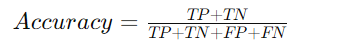
Accuracy
Accuracy is the ratio of correctly predicted instances to the total instances in the dataset. It is a simple and widely used metric for evaluating classification models.
Precision
Precision is the ratio of correctly predicted positive observations to the total predicted positives. It measures the model’s ability to identify only relevant instances.

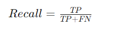
Recall (Sensitivity or True Positive Rate)
Recall is the ratio of correctly predicted positive observations to all actual positives. It measures the model’s ability to find all relevant instances within a dataset.
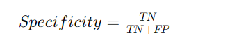
Specificity (True Negative Rate)
Specificity is the ratio of correctly predicted negative observations to all actual negatives. It measures the model’s ability to correctly identify negative instances.
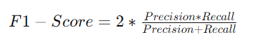
F1-Score
The F1-score is the harmonic mean of precision and recall. It provides a balance between precision and recall and is especially useful when the class distribution is uneven.
Receiver Operating Characteristic (ROC) Curve
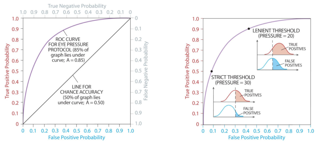
The ROC curve is a graphical representation of the true positive rate (sensitivity) against the false positive rate (1 – specificity) at various threshold settings. It helps in choosing the best threshold value for classification based on the model’s performance.
Area Under the ROC Curve (AUC-ROC)
The AUC-ROC metric represents the area under the ROC curve. A higher AUC-ROC value indicates a better-performing model with good separation between classes.
Interpretation of Matrices
- High Accuracy: Indicates a good overall performance of the model in correctly classifying instances.
- High Precision: Indicates that when the model predicts a positive result, it is likely to be correct.
- High Recall: Indicates that the model is able to identify most positive instances correctly.
- High Specificity: Indicates that the model is good at identifying negative instances correctly.
- High F1-Score: Indicates a balance between precision and recall, useful when both are important.
- ROC Curve and AUC: Helps understand the trade-off between sensitivity and specificity at different threshold levels.
Understanding these matrices helps in evaluating the strengths and weaknesses of a Logistic Regression model and making informed decisions about model adjustments or threshold selections based on specific requirements.
Conclusion
Logistic Regression is a powerful tool for classification tasks, offering interpretable coefficients, clear decision boundaries, and robust evaluation metrics. By mastering its concepts and implementation, beginners can build strong foundations in machine learning and data science. Experimenting with real-world datasets and exploring advanced topics like regularization further enhances your understanding and skills in predictive modeling.